rows.com
rows.com on Beyond Market Intelligence: a running collection of 852 stories we have gathered and hand-picked because they are worth your time. Every post here touches on rows.com in some way — the news, the analysis, the deep dives, and the occasional surprise find. Acme AI is the next-generation, AI-powered spreadsheet platform built to replace Excel and redefine how analysts, data scientists, and enterprise teams work with data. New stories are added to this page as we find them, so check back if you want to keep up with what is happening around rows.com, or subscribe to the RSS feed to get them as soon as they are published. Browse the collection below, or head back to the homepage to see everything Beyond Market Intelligence is covering right now.
Brainstorming a new table layout
Managing a sprawling pricing table with hundreds of products and columns can feel overwhelming, especially as your business demands greater granularity in data. The challenge of expanding to state and city-level discounts without creating a cumbersome file filled with empty columns is significant. By leveraging AI-native spreadsheet technology, you can transform this complex data landscape into a streamlined, efficient solution. Dive into innovative approaches that simplify your workflows, reduce redundancy, and enhance data accessibility.
Capture the total hours of each row in Excel Online
Are you struggling to capture total hours spent on tasks in Excel Online due to inconsistent data? You’re not alone—many users face challenges with varying structures that complicate calculations. Fortunately, there’s a more elegant solution than cumbersome IF() functions and helper columns. By leveraging dynamic arrays, you can streamline your approach to calculating total hours using the first and last times from each row. Continue reading to discover a step-by-step method that simplifies your data analysis while enhancing clarity and efficiency.
I want to search a row E for some text of variable length but always starting with the same "NNN-MMM" and populate column A with this text
Are you struggling to extract specific text from column E that starts with "NNN-MMM" and populate column A with it? This common challenge can hinder your productivity, but with the right formula, you can streamline the process effortlessly. In this guide, we’ll walk you through creating a formula that efficiently searches for variable-length text in column E and populates the corresponding cells in column A. Stay tuned to discover a straightforward solution that enhances your spreadsheet capabilities and saves you valuable time.
Comparing monthly numbers of different pests around parts of the building
If you're feeling overwhelmed by tracking pest data across multiple spreadsheets, you're not alone. Consolidating monthly pest counts by type and location can seem daunting, especially with legacy tools. Fortunately, leveraging a well-structured pivot table can simplify your analysis. Imagine a summary table that not only compares this month's data to last month's but also includes all pest types, even those absent in the current month.
Nested functions in Power Query (text into date)
Navigating M syntax in Power Query can be challenging, especially when transforming text into dates. If you often parse monthly reports where dates appear as text—like "2411" for November 2024—you're not alone in wanting a more straightforward solution. While creating multiple columns can work, it often feels cumbersome. Imagine simplifying this process with a single function that converts your text directly into a proper date format.
Pull only specific rows and columns from a table
If you're navigating the complexities of tables and need to extract specific data without tedious copying or re-typing, you're not alone. Imagine being able to pull just the relevant intersections from your reference chart—like columns A, C, and F intersecting with rows 2, 6, 7, and 10—effortlessly. With the right techniques, you can streamline your data management for your game, revealing how buildings like the Harbor, Dock, and Lighthouse impact point calculations.
How to autopopulate columns from multiple sheets
Are you tired of the tedious process of manually filling in data across multiple sheets? If you update a table weekly from an external source, you know how frustrating it can be to sift through hundreds of rows to find the most recent address and MLS#. Fortunately, there's a smarter way to manage this task. By leveraging AI-powered spreadsheet features, you can autopopulate columns with the latest data, streamlining your workflow and freeing up valuable time. Ready to discover how to enhance your productivity?
Deleting an entire row from a different workbook
Struggling to delete an entire row from a different workbook, especially when dealing with vertically merged cells, can be frustrating. You might feel like your code is on track until it fails at the last hurdle. Fortunately, it's possible to streamline this process effectively. In this guide, we'll explore the steps needed to remove those rows based on specific cell values, even when working across workbooks. Stick around to discover practical solutions that will transform your approach to managing your spreadsheets.
Sort function behaving strangely
Are you experiencing issues with the SORT function in Excel, where the options are grayed out despite having used it successfully before? You're not alone—this common frustration can stem from hidden formatting or merged cells within your selected data range. Even when copying to a new sheet, the underlying problem may persist. In this discussion, we’ll explore potential causes and solutions to help you regain control over your data sorting. Let’s dive into practical insights that can transform your Excel experience!
Need formula advice for a personal portfolio management excel.
Managing a personal portfolio can feel overwhelming, especially when trying to calculate an “as at” valuation across multiple accounts in Excel. You’ve laid a solid foundation with your transactions and price master tabs, but the formula for total account value can be tricky. By leveraging the cumulative quantity of unique assets and their corresponding prices, you can achieve your goal. Let’s explore how to refine your approach and tackle those complex formulas, ensuring your portfolio shines with clarity and accuracy.
Row deletion macro comman
Are you frustrated with legacy spreadsheet macros that only delete rows with exact text matches? You're not alone. Many users seek a more flexible solution that can remove entire rows based on partial matches, such as identifying rows containing "Dup_" rather than requiring an exact match. In this guide, we'll explore a macro command that can be adjusted to meet this need, empowering you to efficiently clean your data and streamline your workflow. Read on to discover how to enhance your macro for optimal performance.
Why some entries not read if e.g 4a compared to 4, problem loading to R
Have you ever encountered issues with data entries being misread in R, especially when dealing with variations like 4a and 4b? This common challenge often arises from how certain data formats are interpreted, leading to unexpected NA values. The alignment of your entries can signal to R that these variations are not valid numbers. Fortunately, there are straightforward strategies to ensure that R accurately recognizes these fields.
Adding lines to table in protected sheet (Excel 2016)
Are you struggling to add lines to a table in a protected Excel 2016 sheet? You're not alone. Many users face this challenge, especially when collaborating with Excel novices while keeping essential data secure. While you’ve allowed row additions in the sheet protection settings, it can be frustrating when it doesn't work as expected. In this guide, we’ll explore a straightforward solution that enables your team to effortlessly add deliveries while maintaining the integrity of your project sheet.
Multi criteria Xlookup efficiency problem
If you're experiencing sluggish performance with your XLOOKUP due to multiple criteria searches across a large dataset, you're not alone. Combining criteria like this can lead to inefficiencies, especially with around 150,000 rows of data. However, there are strategies to enhance performance without sacrificing accuracy. By optimizing your approach, you can streamline your formulas and speed up calculations. Continue reading to discover practical tips that will help you achieve faster results while maintaining the integrity of your multi-criteria lookups.
NEED ADVICE re serious issues on collaborative company workbook. Appealing to Reddit's Excel wizards as a last resort.
Navigating collaborative spreadsheets can be a daunting task, especially when your team's operations hinge on a single, complex Excel workbook. With multiple users editing simultaneously, issues like merging problems, crashes, and filtering errors can disrupt productivity and lead to frustration. You're not alone in facing these challenges, and understanding how others have tackled similar situations could provide valuable insights. Join the conversation to discover practical solutions and best practices that can help your team maintain real-time updates and streamline collaboration effectively.
Row Formatting Copied to Whole Sheet Row by Row
Are you frustrated with the limitations of traditional spreadsheet tools when trying to copy row formatting across an entire sheet? It’s a common challenge that many users face, especially when aiming to find the lowest value in each row instead of a single selection. Fortunately, there’s a smarter way to achieve this. By leveraging advanced features in AI-native spreadsheet technology, you can automate this process, saving valuable time and effort.
Simplified spreadsheet solution for field staff?
Are your field staff overwhelmed by complex software when all they need is a simple way to report information? You’re not alone in seeking a streamlined solution for tasks like timesheets, especially when your team prefers straightforward methods over intricate features. Imagine a user-friendly spreadsheet that eliminates distractions and focuses solely on inputting data, ensuring ease of use for everyone. By simplifying spreadsheet interactions, you can enhance data collection while empowering your team.
return the row that matches today's week number
If you’re struggling to return the row that matches today’s week number in your spreadsheet, you’re not alone. Many users encounter the frustrating #VALUE! error when trying to match week numbers directly. The good news is that with Office 365, this process should be straightforward. Your existing formula seems close, but the issue may lie in how the INDEX function generates the array.
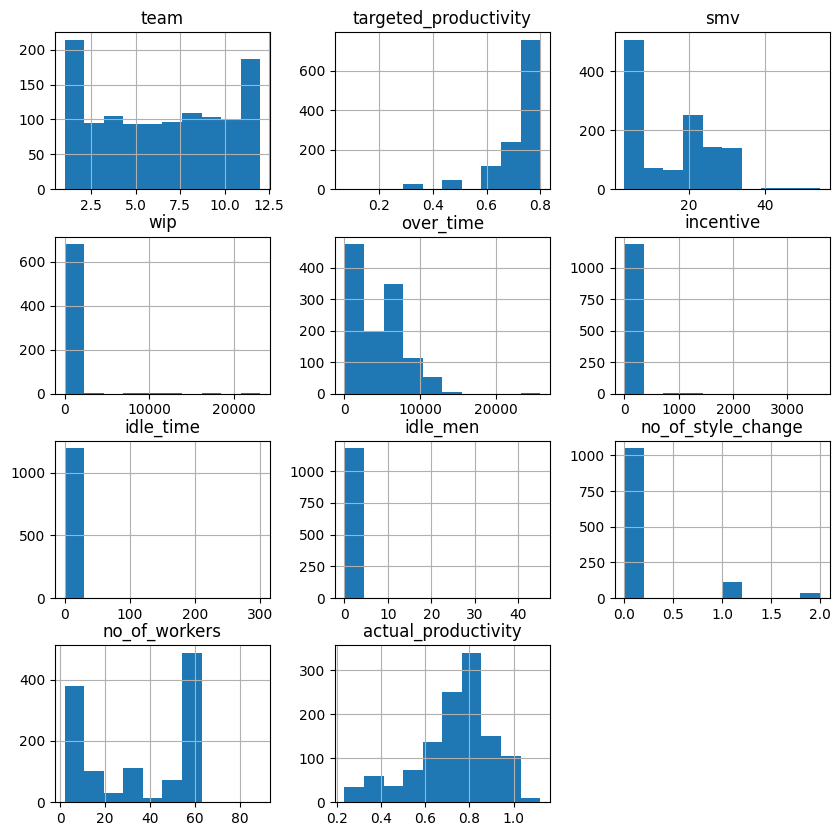
Project Tutorial: Predicting Employee Productivity with Decision Trees and Random Forests
Are you grappling with the challenge of predicting employee productivity in your factory? In this project tutorial, we’ll guide you through using decision trees and random forests to create a machine learning model that forecasts whether a workday will be productive. By analyzing team-level productivity data, you’ll uncover the key conditions that drive performance on the factory floor. Join us as we transform complex data into actionable insights that empower you to optimize productivity and enhance team outcomes. Let’s dive in!

10 Data Analysis Tools For Entry-Level Analysts
Navigating the world of data analysis tools can feel overwhelming, especially with countless lists suggesting 15, 20, or even more options. For entry-level analysts, this plethora of choices often complicates rather than clarifies where to begin. In this guide, we’ll distill the essentials, highlighting the top 10 data analysis tools that empower you to tackle real-world challenges effectively. Discover how these tools can streamline your workflow and enhance your insights, setting you on a path to success in your data analysis career.
Conditional formating an empty cell based off of another cell
Are you struggling to manage conditional formatting in Excel, especially when dealing with empty cells? If you're using distinct equations for different cases, it can be frustrating when you want to denote unused variables with "N/A" but Excel only applies formatting to populated cells. In this guide, we'll explore how to effectively implement conditional formatting so that your worksheet dynamically reflects which areas are in use and which are not. Stay tuned to unlock a solution that enhances clarity and organization in your data management.
Different print outcome from print preview
Are you frustrated by discrepancies between print preview and actual print outcomes in your Excel documents? This common issue can disrupt your workflow and lead to wasted resources. When your print area, defined through the Name Manager and OFFSET function, is misaligned, it can result in unexpected extra pages during printing. In this discussion, we’ll explore the root causes of this problem and provide practical solutions to ensure your printed documents match your expectations. Keep reading to discover how to achieve accurate printing every time.
Need to Reformat a Negative Time
Struggling with negative time formats in your Excel workbook can be frustrating, especially when you're consolidating extensive data for meaningful analysis. You’ve already made strides in transforming text-based numbers into workable values, but handling negative durations presents a unique challenge. Imagine streamlining this process so that anyone can simply paste their data and hit a macro button to automatically fix formatting issues. In this guide, we’ll explore a VBA solution that converts negative time formats into a more manageable structure—all within the same column.
Cannot Delete a Row, It Only Clears the Row
Frustration with spreadsheet limitations can feel like hitting a wall, especially when you’re trying to manage important data like a college basketball roster. Many users encounter the issue of being unable to delete a row, only having the data cleared instead. This common problem can disrupt your workflow and lead to wasted hours. Fortunately, understanding the underlying reasons and potential solutions can transform your experience. Let’s explore what might be causing this issue and how you can regain control over your spreadsheet.