rows.com
876 stories filed under rows.com on Beyond Market Intelligence. The newest of them: “How React Server Components expose a critical deserialization risk”, “Predict your spreadsheet data with a simple click, no code required.”, and “Transform uncategorized data into clarity with automated category assignment.”. React Server Components promise a smoother path to interactive UIs, but that same Flight protocol hands attackers a surprisingly deep bag of tricks. TabFM Studio puts tabular foundation models directly on your desktop, no code required. Acme AI is the next-generation, AI-powered spreadsheet platform built to replace Excel and redefine how analysts, data scientists, and enterprise teams work… The list below is every rows.com story on Beyond Market Intelligence, newest first.

How React Server Components expose a critical deserialization risk
React Server Components promise a smoother path to interactive UIs, but that same Flight protocol hands attackers a surprisingly deep bag of tricks. Durgesh Pawar digs into the mechanics of "React2Shell," a CVSS 10.0 flaw where deserialization sinks turn protocol manipulation into remote code execution. It is a sharp reminder that convenience often carries hidden weight. For more on turning complex data challenges into practical wins, our piece on deduplicating supplier lists with deterministic stages pairs well with this mindset.
Predict your spreadsheet data with a simple click, no code required.
TabFM Studio puts tabular foundation models directly on your desktop, no code required. Drop in a CSV or Excel file, click the column you want to predict, and let the model fill in the blanks using your existing rows as examples. It's a smart, accessible wrapper around Google's TabFM, built for people who'd rather not wrestle with Python. We've covered similar ground with deterministic deduplication, but this feels like a more natural entry point for everyday spreadsheet users.

Transform uncategorized data into clarity with automated category assignment.
Uncategorized rows quietly undermine a report, and in facility management, that means lost grouping and aggregation. A practical fix exists, and this story walks through how to assign categories automatically using Power Query and DAX. This is a straightforward approach to a recurring problem, and the solution feels immediately applicable. For readers hungry for more analytical problem-solving, the related piece on bridging retrieval and action offers a complementary perspective worth exploring.
Learning Rate Defaults Don't Fit Small Dataset Fine-Tuning
A single learning rate buried in a shared notebook cost someone three weeks of their life. The qlora 2e-4 default is wrong under 10k samples, and nobody talks about it. This user did the hard work of questioning the copy-paste consensus, and they found that dropping to 1e-4 and adding epochs moved the eval more than all their data cleaning combined. That is the practical insight most tutorials skip. If you are fighting small datasets, start lower and tune that one number.

Trust in AI agents is the real barrier to enterprise deployment
The gap between AI agent pilots and production isn't a capability problem; it's a reliability problem. Bryan Silverthorn, Amazon's Director of AGI Autonomy, made that case at VB Transform 2026, pointing to a framework that breaks reliability into consistency, robustness, predictability, and safety. His "intern" analogy is the right way to think about it. Agents need management, not just better benchmarks. For deeper context on navigating these adoption challenges, our related piece, "Unlock AI's Enterprise Potential," offers a broader lens.
Why enterprise AI agents stall at deployment, not capability
At VB Transform 2026, Bryan Silverthorn from Amazon made a pointed case: enterprise AI agents aren't failing because they're not smart enough. They're failing because they're not reliable enough. With 85% of companies piloting agents but only 5% shipping them, the gap is a measurement problem, not a model problem. His "intern" framework is a refreshingly human lens on managing autonomous systems. It's practical advice for escaping pilot purgatory. For more on scaling these workflows, see our piece on orchestrating AI agents with Google's AX.

ChatGPT Work turns your AI assistant into an autonomous task manager
OpenAI introduces ChatGPT Work, a cloud-based AI agent poised to transform how professionals leverage AI. Embedded within the flagship chatbot, this new platform moves beyond simple Q&A, autonomously managing tasks across email, Slack, and calendars using the advanced GPT-5.6 model. ChatGPT Work streamlines workflows by generating documents, spreadsheets, and even websites, demonstrating OpenAI's commitment to democratizing agentic AI capabilities – a strategy highlighted by their recent confidential SEC filing.

Google's TabFM predicts on unseen tables without per-dataset training.
Google Research’s TabFM offers a transformative approach to tabular data prediction, bypassing the traditional need for per-dataset training. This innovative foundation model treats tabular prediction as an in-context learning problem, enabling instant predictions on unseen tables with a single API call – a significant acceleration for enterprise developers. By synthesizing strengths from prior architectures, TabFM preserves data structure and unlocks scalable zero-shot prediction, potentially redefining data workflows.

Your Data Stays Local as AlloyDB Runs AI Queries at Database Speed
Google's AlloyDB AI functions are now generally available, introducing a transformative approach to AI-powered data management. This innovation utilizes proxy models—lightweight, locally trained versions of large language models—to execute queries directly within the database, eliminating external calls and dramatically accelerating performance. Early internal testing demonstrates a remarkable 2,400x throughput improvement, achieving speeds up to 100,000 rows per second. For further insights into real-time systems, explore our related article, "Beat-Aligned Mobile Audio Streaming with Virtual Chunks and Native Playback."

Break Free from the Box with WordPress's First Infinite Canvas Builder
For years, WordPress website design has been constrained by rigid templates. Now, meet Kirki, the first freeform visual builder offering an infinite canvas. This innovative tool redefines the WordPress experience with cleaner performance and unparalleled design freedom—all without plugin dependency. Discover a more intuitive workflow and unlock your creative potential. Explore Kirki and elevate your website building. For deeper insights into scaling complex systems, see our article on "How HubSpot Scaled Semantic Search to 20 Billion Vectors."
Comparing small TTS models side by side with objective MOS benchmarks
Evaluating small text-to-speech (TTS) models requires careful benchmarking, and we’ve compiled a CPU-based assessment of Kokoro, Supertonic, Inflect-Nano, and Kyutai’s Pocket TTS. Utilizing UTMOS MOS scoring across 180 runs on an Intel Xeon platform, our findings reveal interesting performance nuances, particularly regarding Pocket TTS's consistent RTF scaling and the limitations of UTMOS in assessing smaller vocoders.
Discover how flexible text matching simplifies your spreadsheet workflows.
To accommodate users belonging to multiple regions, your existing formula requires modification. Given your preference for a single "Region" column with delimited values (e.g., "Hawaii and Okinawa"), adjust the formula in column V to: `=IF(AND(ISNUMBER(SEARCH(V$36,C39)),NOT(V$36="")),"Yes","")`. This utilizes the `SEARCH` function, which returns a number if the text in V$36 is found within C39, enabling partial matches. For the "Region 2" column approach, a similar formula can be applied to the new column, referencing the appropriate region field. See
Simplify complex conditional checks with smarter spreadsheet logic
To efficiently identify "ending" rows in your spreadsheet where preceding tasks remain incomplete, leverage conditional formatting. Specifically, flag the "ending" row if *any* corresponding month’s tasks have a FALSE value in column I. This can be achieved with a formula examining column I for TRUE values within the relevant date range. Consider a helper column (column J) for clarity, though it's possible to maintain your existing formulas in columns H-I.
Track projects with clarity and keep notes right where they belong
Managing a growing project list—particularly when physical printouts are essential—demands a thoughtful approach. For users familiar with traditional spreadsheets, transitioning to a system that balances data organization with readability is key. Our solution allows you to track project details (budget, status, action items) in a standard row, while maintaining dedicated notes below each project. Critically, this design preserves sortability by project information while optimizing print clarity.
Tame uneven data sets with a smarter approach to capital gain reconciliation
Reconciling capital gains statements with mismatched data sets can be challenging, especially when dealing with data from disparate sources. As a junior accountant, you're right to seek efficient solutions beyond manual processes. For smaller datasets (100-200 rows), leveraging Excel’s lookup functions—even with data misalignment—is a viable approach. Focus on establishing a clear mapping between the Capital Gain Statement and the Annual Information Statement columns, then utilize lookup formulas to align the data.
From kitchen chaos to prep clarity with smarter sales data
Navigating complex food and beverage sales data can be challenging, especially when aiming for streamlined ordering and prep. You’ve already made significant progress by automating data import from Square using Power Query and Pivot Tables—a key step toward a future-focused, efficient workflow. Now, the goal is to distill this data into a clear “sales per 1k guests” metric on your dashboard. As you explore this, consider the strategies outlined in our article, "Excel Spreadsheet to organize my Pills/Supplements," for managing and tracking data effectively.
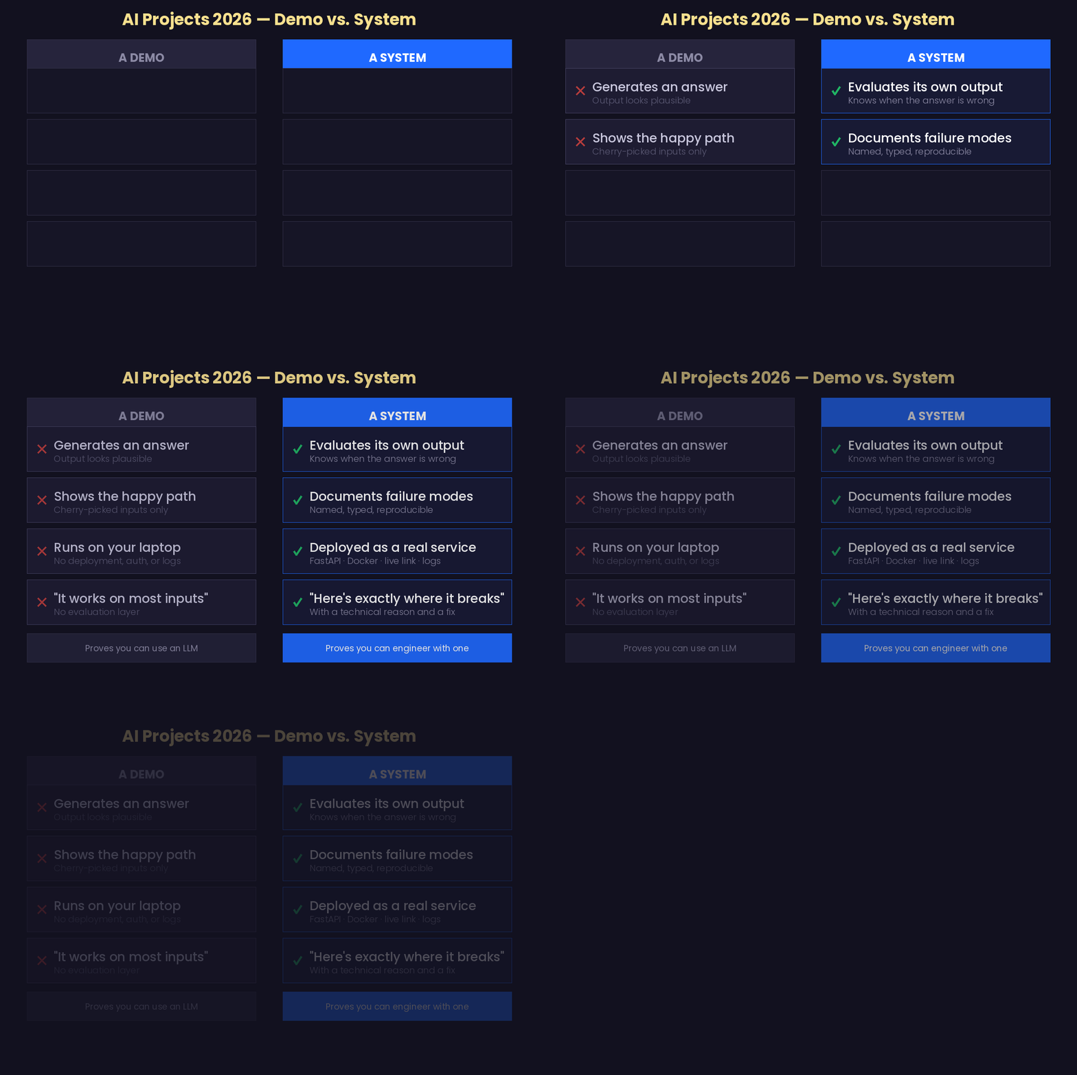
Build AI projects that prove you know where your system fails
Navigating the landscape of AI projects for 2026 requires a focused approach. The most compelling projects aren't about sheer complexity; they're about demonstrating a clear understanding of system limitations and articulating those failures confidently to potential employers. Forget wading through 50 ideas – this post delivers the top 10 AI projects poised to impress. Discover how to build demonstrable skills and showcase your expertise. For deeper insights into user interface design within AI, explore "Matching AI Modality To User Intent."
Track every row change and roll back with a simple dropdown
Maintaining a detailed audit trail for frequently updated spreadsheet rows is crucial for data integrity. To empower users like /u/bigdeekenergy, who manage document trackers with numerous revisions, consider implementing a system where each row’s history is readily accessible. Our approach prioritizes clarity: a dropdown menu, specific to each row, would display only its previous versions, allowing for easy review and, ideally, selective rollback of individual cells.

Design AI interfaces around user intent, not just chat
The rush to integrate AI often defaults to chat interfaces, overlooking a fundamental principle of user experience: matching modality to intent. Simply because Large Language Models thrive on dialogue doesn’t mean every AI capability should be presented conversationally. Great UX prioritizes the user, adapting the interface to their context and cognitive load. Explore how shifting beyond conversational tunnel vision unlocks more intuitive and effective data interactions—as discussed further in "Users Don’t Need More Tools: They Need Seamless Integrations."
Forecasting Air Quality Across Chaos with Smarter Data Models
This project delivers a globally accurate Air Quality (PM2.5) forecasting model across the US, UK, India, and Australia, addressing a critical challenge: variance. Initial models struggled in regions with high volatility, performing worse than naive carryover predictions. The solution? A horizon-aligned architecture decoupling forecast horizons and incorporating a volatility matrix to prevent data leakage. Achieving a consistent MASE below 1.0, even at a 30-day horizon, demonstrates a 57% predictive accuracy improvement. See "Time Series Modeling Needs a Dynamical Systems Perspective" for related insights. [https://global-aq-intelligence.vercel.app/](https://global-

Your AI agent framework just handed attackers your keys.
Three widely deployed AI agent frameworks – LangGraph, Langflow, and LangChain – share a critical vulnerability, exposing sensitive data like OpenAI keys, database credentials, and CRM tokens. Recent attacks exploiting a SQL injection in LangGraph and a path traversal in Langflow demonstrate that these frameworks, adopted rapidly, have outpaced security measures. Now, researchers have identified a similar flaw in LangChain-core. Addressing this requires immediate action: patching to the latest versions and reviewing framework configurations to minimize exposure.

Enterprise AI's open door: why trust boundaries matter now
Enterprise AI is rapidly expanding, but a concerning pattern is emerging: external input is being accepted without robust trust boundaries. Recent disclosures like SearchLeak (affecting Microsoft Copilot) and vulnerabilities in LiteLLM highlight this risk. Four independent teams have now uncovered similar flaws across diverse tools, demonstrating a systemic operating failure. This five-check trust-boundary audit maps these gaps to concrete actions, allowing you to proactively address vulnerabilities and communicate risks clearly to your board—starting before lunch.

How AI agents finally killed the data pipeline bottleneck
For decades, data professionals have grappled with unifying operational and analytical databases—a challenge now acutely amplified by the demands of AI agents. Databricks is addressing this structural problem with Lakehouse//RT and LTAP, aiming to eliminate the latency and complexity of traditional data pipelines. Lakehouse//RT delivers millisecond query speeds directly on governed data, while LTAP stores transactional data in Delta and Iceberg format.

Why RAG Fails at Aggregation and How to Fix It
Traditional approaches to Retrieval-Augmented Generation (RAG), like simply expanding context windows, often fail to improve accuracy—and can even mask errors—when dealing with aggregation tasks. Our recent analysis, benchmarking RAG pipelines against a full-scan engine across a substantial dataset, reveals a critical limitation: computation queries should be rerouted entirely. Explore how we've built a system to address this, offering a more reliable solution. For deeper insights into related challenges facing AI developers, see our article on Anthropic's recent restrictions.